In the coming months, I’ll prepare some tutorials over an excellent data analysis package called pandas !
To show you the power of pandas, just take a look at this old tutorial, where I exploited the power of itertools to group sparse data into 5 seconds bins.
The magic of pandas is that, when you two arrays, “times” and “values”, then you can create a DataFrame of values, indexed by times. Once this is done, you can resample the index array and choose a grouping function (“mean”, “sum” or pass a function: np.sum, np.median, etc…).

Once the times array was defined, the core of the code was :
SECOND = 1
MINUTE = SECOND * 60
HOUR = MINUTE * 60
DAY = HOUR * 24

binning = 5*SECOND

def group(di):
    return int(calendar.timegm(di.timetuple()))/binning

list_of_dates = np.array(times,dtype=datetime.datetime)
grouped_dates = [[datetime.datetime(*time.gmtime(d*binning)[:6]), len(list(g))] for d,g in itertools.groupby(list_of_dates, group)]
grouped_dates = zip(*grouped_dates)

plt.bar(grouped_dates[0],grouped_dates[1],width=float(binning)/DAY)
Now, doing the same with pandas is … only 4 lines of code…
binning=5
dt = pd.DataFrame(np.ones(N),index=times)
rs = dt.resample("%iS"%binning,how=np.sum)
rs.plot(kind='bar')
And the whole code could even be shorter by using pandas’ built-in functions to create date/time spans etc…
The full code is after the break:
import numpy as np
import matplotlib.pyplot as plt
import datetime, time, calendar
from matplotlib.dates import num2date, DateFormatter
import pandas as pd
N = 100000
binning = 5
starttime = time.time()
basetimes = sorted(np.random.random(N)*np.random.random(N)*1.0e3+starttime)
times = [datetime.datetime(*time.gmtime(a)[:7]) for a in basetimes]
for i, atime in enumerate(times):
times[i] = atime + datetime.timedelta(microseconds=(basetimes[i]-int(basetimes[i])) * 1e6)
dt = pd.DataFrame(np.ones(N),index=times)
rs = dt.resample("%iS"%binning,how=np.sum)
rs.plot(kind='bar')
plt.grid(True)
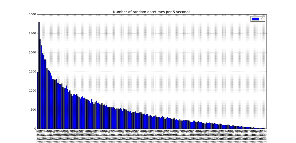
plt.title('Number of random datetimes per %i seconds' % binning)
plt.show()