Imagine we want to plot a map of the seismic activity in NW-Europe and, at the same time, count the number events per month. To get a catalogue of earthquakes in the region, one can call the NEIC (note: this catalogue contains a lot of different stuff, i.e. quarry blasts, mining-induced events, army-directed WWI&II bombs explosions at sea, etc). Anyway, it’s a BIG dataset, big enough to justify an automated mapping & rate estimation script !
The goal:
Obtaining

Process:
First, we’ll get the catalogue from NEIC, by calling their search page directly (not sure it’s the best way…):
request = """http://neic.usgs.gov/cgi-bin/epic/epic.cgi?
SEARCHMETHOD=2&FILEFORMAT=4&SEARCHRANGE=HH
&SLAT2=54&SLAT1=45&SLON1=-5&SLON2=15
&SYEAR=&SMONTH=&SDAY=&EYEAR=&EMONTH=&EDAY=
&LMAG=&UMAG=&NDEP1=&NDEP2=&IO1=&IO2=
&CLAT=0.0&CLON=0.0&CRAD=0.0&SUBMIT=Submit+Search"""

import urllib
u = urllib.urlopen(request)
lines = u.readlines()[34:-33]

events = [line.split()[1:9] for line in lines]
in this code, we get the data using urllib by passing a long request containing our zone of interest (defined in line 3 of the request). The output is then sliced to reject header and footer, then splitted into chunks containing the information of each event.
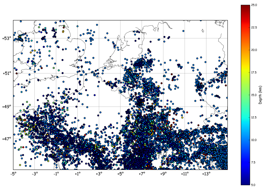
The map is drawn using:
ye,mo,d,t,lat,lon,dep,mag = zip(*events)
lon = np.array(lon,dtype='float')
lat = np.array(lat,dtype='float')
dep = np.array(dep,dtype='float')
x,y = m(lon,lat)
plt.scatter(x,y,c=dep,vmin=5,vmax=25)
cb = plt.colorbar()
cb.set_label('Depth (km)')
plt.show()
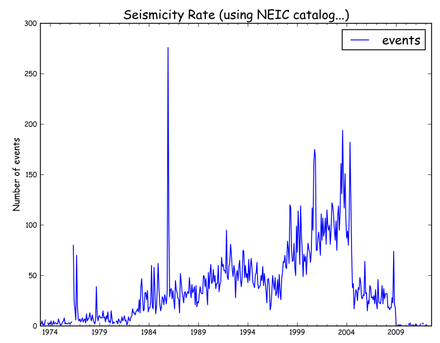
while the seismicity rate is computed and plotted using pandas:
dates = []
for yi, moi, di, ti in zip(ye,mo,d,t):
    date = "%04i-%02i-%02i %s" % (int(yi), int(moi), int(di),ti[0:6])
    date = datetime.datetime.strptime(date,'%Y-%m-%d %H%M%S')
    dates.append(date)

df = pd.DataFrame({"events":np.ones(len(dates))},index=dates)
rs = df.resample('1M',how='sum')
rs.plot()
plt.title('Seismicity Rate (using NEIC catalog...)')
plt.ylabel('Number of events')
plt.show()
In this case, we resample the index (= the dates) to 1 value per month. The resampling is done using how=”sum”, telling pandas to count the number of events (each event is a 1 in the DataFrame).
And… It’s done !
From a seismological point of view:
The apparent increase in rate from 1997 onwards could be related to either: a change in magnitude threshold sent by networks or agencies to the NEIC, a change in filtering of events (quarry blasts, etc), or a real rate increase. The drop after 2004 could have the same reasons, but in opposite direction. Those ideas will be treated in the next tutorials, stay tuned !
For sure, most of the earthquakes located in the centre of the Ardenne (SE Belgium) are mostly quarry blasts. We’ll show how to determine that in another tutorial, too !
The full code is after the break:
#
# Basemap & Pandas example by geophysique.be
# tutorial 1

import numpy as np
import matplotlib.pyplot as plt
from mpl_toolkits.basemap import Basemap
import urllib
import datetime
import pandas as pd

### PARAMETERS FOR MATPLOTLIB :
import matplotlib as mpl
mpl.rcParams['font.size'] = 12.
mpl.rcParams['font.family'] = 'Comic Sans MS'
mpl.rcParams['axes.labelsize'] = 10.
mpl.rcParams['xtick.labelsize'] = 8.
mpl.rcParams['ytick.labelsize'] = 8.

fig = plt.figure(figsize=(11.7,8.3))
#Custom adjust of the subplots
plt.subplots_adjust(left=0.05,right=0.95,top=0.90,bottom=0.05,wspace=0.15,hspace=0.05)
ax = plt.subplot(111)
#Let's create a basemap of NW Europe
x1 = -5.0
x2 = 15.
y1 = 45.
y2 = 54.

m = Basemap(resolution='i',projection='merc', llcrnrlat=y1,urcrnrlat=y2,llcrnrlon=x1,urcrnrlon=x2,lat_ts=(y1+y2)/2)
m.drawcountries(linewidth=0.5)
m.drawcoastlines(linewidth=0.5)
m.drawparallels(np.arange(y1,y2,2.),labels=[1,0,0,0],color='black',dashes=[1,0],labelstyle='+/-',linewidth=0.2) # draw parallels
m.drawmeridians(np.arange(x1,x2,2.),labels=[0,0,0,1],color='black',dashes=[1,0],labelstyle='+/-',linewidth=0.2) # draw meridians

request = """http://neic.usgs.gov/cgi-bin/epic/epic.cgi?SEARCHMETHOD=2&FILEFORMAT=4&SEARCHRANGE=HH
&SLAT2=54&SLAT1=45&SLON1=-5&SLON2=15
&SYEAR=&SMONTH=&SDAY=&EYEAR=&EMONTH=&EDAY=
&LMAG=&UMAG=&NDEP1=&NDEP2=&IO1=&IO2=
&CLAT=0.0&CLON=0.0&CRAD=0.0&SUBMIT=Submit+Search"""

u = urllib.urlopen(request)
lines = u.readlines()[34:-33]

events = [line.split()[1:9] for line in lines]

ye,mo,d,t,lat,lon,dep,mag = zip(*events)
lon = np.array(lon,dtype='float')
lat = np.array(lat,dtype='float')
dep = np.array(dep,dtype='float')
x,y = m(lon,lat)
plt.scatter(x,y,c=dep,vmin=5,vmax=25)
cb = plt.colorbar()
cb.set_label('Depth (km)')
plt.savefig('event_map.png',dpi=300)
plt.show()

dates = []
for yi, moi, di, ti in zip(ye,mo,d,t):
    date = "%04i-%02i-%02i %s" % (int(yi), int(moi), int(di),ti[0:6])
    date = datetime.datetime.strptime(date,'%Y-%m-%d %H%M%S')
    dates.append(date)

df = pd.DataFrame({"events":np.ones(len(dates))},index=dates)
rs = df.resample('1M',how='sum')
rs.plot()
plt.title('Seismicity Rate (using NEIC catalog...)')
plt.ylabel('Number of events')
plt.savefig('event_rate.png',dpi=300)
plt.show()

Hi there,
I just found your blog and I really like your examples, looking forward for more pandas stuff!
Benjamin
Thanks !!
x,y = m(lon,lat)
m is not defined
look at the full code at the bottom of the plot, m is defined (not in the chunks above).